Introduction
The secpRod package provides a number of methods to
calculate secondary production of populations, both those with clear
cohort structure and those where cohort structure is not possible to
discern. First, we walk through the available methods using simulated
populations that mimic the data structure of real sampling regimes. The
parameters to create these simulated populations is outlined in
companion article, “Simulating
the sampling of populations” vignette. These simulated populations
skip some of the steps of moving from initial sampling processes (e.g.,
length to mass conversions, sample subsetting, etc.) that are often part
of the process. More complete examples that showcase helper functions
within secpRod that deal with these processes can be found
below in the “A
full example” vignette. Here, we just showcase the secondary
production methods available.
The methods within the package use two main objects,
sampleInfo the sample-level information (e.g., site, date ,
replicate) and density and length or mass. An additional dataframe,
taxaInfo that houses species-specific information such as
length to mass conversions, and method specific information such as
cohort production interval estimates (CPIs), production:biomass ratios
(PBs), and growth equations. The columns contain information for the
calculation of production. These include, but are not limited to:
taxonID: a character string that matches the name of taxonID from sampleInfo
massForm: a character string that is coercible to a formula for the conversion from length to mass (e.g.,
mass~(a*lengthClass^b))a: numeric variable for the coefficients used in massForm
b: numeric variable for the coefficients used in massForm
percAsh: numeric integer 0–100
-
method: character string for the method to use. Must be one of the following:
- ‘is’: increment-summation method. This cohort-based method calculates interval and annual production, , from field data as the sum of all interval production, , plus initial biomass, :
‘rs’: removal-summation method is similar to the increment-summation method but instead calculates the production lost during a sampling interval as the product of the decrease in density, and the mean individual mass, plus the increase in biomass, .
‘sf’: size-frequency method. This non-cohort approach assumes the mean size-frequency data from collected samples characterizes the mortality, growth and development of an average cohort. The densities within size classes are averaged across all sampling dates and the decrease in density across sizes classes is calculated similar to the removal-summation method. This method assumes a 1-year lifespan. If taxa have an average life span much shorter or longer than 1-year, a cohort production interval (CPI) correction must be applied. See Benke (1979) or Benke and Huryn (2017) for a more complete explanation. The CPI must be provided in the
min.cpiandmax.cpivariables of thetaxaInfoobject.‘igr’: instantaneous growth method. This approach is most often applied as a noncohort approach, but can also be used for taxa with identifiable cohorts. It requires the determination of daily instantaneous growth rates, g_d, specified in
growthForm. Growth rates can be determined through a number of approaches such as, from growth chambers in the field or laboratory, mark-recapture of individuals, or statistical regression models. See Huryn and Wallace (1986), Morin and Dumont (1994), Benke and Huryn (2017) and the citations therein for more examples of these approaches.‘pb’: production:biomass ratio method. This approach calculates production by multiplying annual biomass by a value of production:biomass ratio (P:B). The P:B must be supplied in the
pbvariable of thetaxaInfoobject.
growthForm: daily growth rates, g_d, to calculate production from the instantaneous growth method. This takes the form of a character string that is coercible to a formula. This formula is parsed and will, if necessary, reference existing information (e.g., size information) if variables are included in the formula. The variables in the string must match exactly those in the data (e.g., if massValue == ‘mass’, ‘mass’ must be in the dataframe). Warning: this method is currently under development to include additional sources of environmental data (e.g. temperature). When complete, additional data passed to
envDatawill also be referenced to predict growth rates. Currently, the tests for this feature are still in development, it will not reject any nonsensical values (e.g, negative, NA, or Inf). If your equation predicts negative values you may get negative production estimates–at least until themin.growthfeature is implemented.min.cpi: integer of the minimum estimated cohort production interval for adjusting annual production estimates using the size-frequency method
max.cpi: integer of the maximum estimated cohort production interval for adjusting annual production estimates using the size-frequency method
pb: numeric of the production to biomass (PB) ratio for the specific taxa. This can take three forms 1) a single value, 2) a vector of values the same length as
bootNum, and 3) a string of a distribution to randomly sample, not including then =(e.g., ‘rnorm(mean = 5, sd = 0.5)’, ‘runif(min = 3, max = 8)’). The function will automatically sample thebootNumvalues. Warning: Currently, you must explicitly name the parameters in the distribution call string (e.g., mean, sd, min, max). Possible unwanted and unknown things will happen otherwise. The tests for this feature are still under development, it will not reject any nonsensical values (e.g, negative, NA, or Inf). If your distribution samples negative values you will get negative production estimates. At least until themin.growthfeature is implemented.min.growth: a minimal growth rate value of g_d to assign when density is >0 and growth estimates for a taxon are <0. This is currently not implemented, but is kept for future use.
wrap: logical (or coercible) indicating whether the production estimate should wrap the first and last dates to create a full annual cycle. If TRUE, this will create an additional sampling interval using the mean densities and masses of the first and last sampling events to create a full annual data set. The default is FALSE.
envData: additional information or data to pass to the function. This is mainly used to pass environmental data to inform growth rate information by included information such as temperature, food availability, etc.
notes: notes for researcher use. This column will be maintained in output summaries.
taxaInfo <- tibble::tibble(
  taxonID = c("sppX"),
  massForm = c("mass~(a*lengthClass^b)*percAsh"),
  # a is NA for this example because we simulated mass growth and don't need to convert from length to mass
  a = c(NA),
  # b is NA for this example because we simulated mass growth and don't need to convert from length to mass
  b = c(NA),
  # percAsh is NA for this example because we simulated mass growth and don't need to convert from length to mass
  percAsh = c(NA),
  # method can accept one or more values. This allow comparisons among different methods.
  method = 'is',#list(c("is","pb","sf")),
  growthForm = c("g_d ~ exp(log(0.01) - 0.25*log(mass) + 0.01*log(tempC))"),
  min.cpi = c(335),
  max.cpi = c(365),
  pb = c("runif(min = 3, max = 8)"),
  min.growth = c(0.001),
  wrap = FALSE,
  notes = c("This is here for your use. No information will be used, but this column will be maintained in some summaries. See *** for more information.")
)
A multi-method comparison with simulated data
First, we load and visualize the simulated cohort data set, which contains a single species and follows the progression of density and the distribution of individual masses through it life cycle.
The data set is available within the secpRod package
with:
data('singleCohortSim', package = 'secpRod')The sampleInfo for this species includes:
#> # A tibble: 10 × 5
#>    taxonID dateID repID  mass density
#>    <chr>    <dbl> <int> <dbl>   <dbl>
#>  1 sppX         1     1 0.001     463
#>  2 sppX         1     2 0.001     458
#>  3 sppX         1     3 0.001     479
#>  4 sppX         1     4 0.001     422
#>  5 sppX         1     5 0.001     639
#>  6 sppX         1     6 0.001     575
#>  7 sppX         1     7 0.001     518
#>  8 sppX         1     8 0.001     677
#>  9 sppX         1     9 0.001     566
#> 10 sppX         1    10 0.001     468
this object can be a data.frame (or coercible) or a tibble (if list-cols are used) which contains the following columns:
taxonID: (required) a character string that matches the name of taxonID from taxaInfo
dateID: a column representing the date identifier. This can be a julian date (as in this case) or a recognized date object (e.g., Date class, POSIXct, etc.)
repID: a column representing the replicate identifier for the length and mass data
density: (or column name specified in
abunValue) organism density of each length or mass class in the replicatemass: (or column name specified in
massValue) individual mass. This is the mass class with a corresponding density. The density of each mass class sums to the total sample density.
These columns names above are the default column names. The exact
names of these some columns (and additional optional columns such as
length information) can be modified within the
calc_production() function. See “A
full example” for more information on customizing this main function
further.
We can summarize and visualize this data set further.
summary_stats <- singleCohortSim %>%
  dplyr::mutate(density = sum(density, na.rm = TRUE), .by = c('taxonID','dateID','repID')) %>%
  dplyr::summarise(
    massMean = mean(mass, na.rm = TRUE),
    massSD= sd(mass, na.rm = TRUE),
    larvalDensityMean = mean(density, na.rm = TRUE), .by = 'dateID'
  )

sim_plot =
ggplot(summary_stats, aes(x = dateID)) +
  stat_halfeye(data = singleCohortSim %>%
                 dplyr::summarise(density = sum(density, na.rm = TRUE), .by = c('taxonID','dateID','repID')), aes(x = dateID, y = density),
               color = 'green')+
  stat_halfeye(data = singleCohortSim, aes(x = dateID, y = mass*100),
               color = 'red')+
  geom_path(aes(y = larvalDensityMean), color = 'green') +
  geom_path(aes(y = massMean * 100), color = 'red') +
  scale_y_continuous(
    name = "Larval Density",
    sec.axis = sec_axis(~./100, name = "Mean Mass (mg)"),

  ) +
  scale_x_continuous(limits = c(0,365))+
  theme_minimal() +
  labs(title = "Larval Density and Mean Mass over Time", x = "Day")+
  theme(axis.title.y.right = element_text(color = 'red'))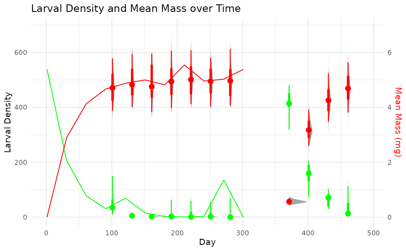
We use this data set to calculate secondary production with different
methods. First, we start with cohort-based methods. The main function of
secpRod is calc_production() which is the
workhorse function that will estimate population and/or community
production.
To apply it to our single species example, we input the sample information and taxa information along with how many bootstraps we would like, as:
calc_production(
  taxaSampleListMass = singleCohortSim,
  taxaInfo = taxaInfo,
  bootNum = 10,
  taxaSummary = TRUE,
  massValue = 'mass',
  abunValue = 'density'
)
This will output an object with bootstrapped estimates as well as a summary of the samples. It has a simple structure:
P.boots–vectors of bootstrapped estimates of annual production, annual mean biomass, and annual mean abundance.
taxaSummary–is a summary of the sampled data, including estimated production, sampling event summaries of density, biomass, and production (if applicable). This can be turned off by setting
taxaSummarytoFALSE.
Below, we walk through each of the available methods using this simulated population. For further details on these methods and their calculations, see (benke2007?).
Increment-summation
set.seed(1312)
calc_production(
  taxaSampleListMass = singleCohortSim,
  taxaInfo = taxaInfo,
  bootNum = 1e1,
  taxaSummary = TRUE,
  massValue = 'mass',
  abunValue = 'density'
)
#> $P.boots
#>            [,1]     [,2]     [,3]     [,4]     [,5]     [,6]     [,7]
#> P.ann.samp 2326.716 1948.697 1972.095 2036.732 2289.194 1911.34  2054.362
#> B.ann.samp 121.7319 98.44109 112.0241 111.5616 111.0987 124.9283 119.6349
#> N.ann.samp 81.54545 76.73636 75.85455 79.63636 80.76364 81.43636 81.39091
#>            [,8]     [,9]     [,10]
#> P.ann.samp 2090.462 1538.009 1659.261
#> B.ann.samp 100.207  82.95062 88.37525
#> N.ann.samp 80.88182 67.33636 76.12727
#>
#> $taxaSummary
#> $taxaSummary$taxonID
#> [1] "sppX"
#>
#> $taxaSummary$method
#> [1] "is"
#>
#> $taxaSummary$P.ann.samp
#> [1] 1965.248
#>
#> $taxaSummary$P.uncorr.samp
#> NULL
#>
#> $taxaSummary$pb
#> [1] 19.01809
#>
#> $taxaSummary$meanN
#> [1] 76.81818
#>
#> $taxaSummary$meanB
#> [1] 103.3357
#>
#> $taxaSummary$meanIndMass
#> [1] 1.345199
#>
#> $taxaSummary$datesInfo
#>    dateID  N density_mean density_sd biomass_mean   biomass_sd
#> 1       1 10        526.5 84.7312746       0.5265   0.08473127
#> 2      31 10        188.3 59.5110634     545.8428 174.77142887
#> 3      61 10         59.7 34.3642256     246.7510 141.80435903
#> 4      91 10         18.2 15.8591018      84.9913  74.46818703
#> 5     121 10         25.8 35.2445425     125.7648 171.92585860
#> 6     151 10          7.0  8.2192187      34.9949  41.35086763
#> 7     181 10          1.4  1.7126977       6.7490   8.13225550
#> 8     211 10          0.3  0.6749486       1.6633   3.68722961
#> 9     241 10          1.1  1.9692074       5.4528   9.50699300
#> 10    271 10         16.6 47.2915308      83.4182 237.84375664
#> 11    301 10          0.1  0.3162278       0.5382   1.70193784
Size-frequency
taxaInfo <- tibble::tibble(
  taxonID = c("sppX"),
  massForm = c("mass~(a*lengthClass^b)*percAsh"),
  # a is NA for this example because we simulated mass growth and don't need to convert from length to mass
  a = c(NA),
  # b is NA for this example because we simulated mass growth and don't need to convert from length to mass
  b = c(NA),
  # percAsh is NA for this example because we simulated mass growth and don't need to convert from length to mass
  percAsh = c(NA),
  # method can accept one or more values. This allow comparisons among different methods.
  method = 'sf',#list(c("is","pb","sf")),
  growthForm = c("g_d ~ exp(log(0.01) - 0.25*log(mass) + 0.01*log(tempC))"),
  min.cpi = c(290),
  max.cpi = c(310),
  pb = c("runif(min = 3, max = 8)"),
  min.growth = c(0.001),
  wrap = FALSE,
  notes = c("This is here for your use. No information will be used, but this column will be maintained in some summaries. See *** for more information.")
)

set.seed(1312)
calc_production(
  taxaSampleListMass = singleCohortSim,
  taxaInfo = taxaInfo,
  bootNum = 2,
  taxaSummary = TRUE,
  massValue = 'mass',
  abunValue = 'density'
)
#> $P.boots
#>               [,1]     [,2]
#> P.ann.samp    5181.701 5010.692
#> P.uncorr.samp 4131.164 4008.554
#> B.ann.samp    121.7319 98.44109
#> N.ann.samp    81.54545 76.73636
#>
#> $taxaSummary
#> $taxaSummary$taxonID
#> [1] "sppX"
#>
#> $taxaSummary$method
#> [1] "sf"
#>
#> $taxaSummary$P.ann.samp
#> [1] 6230.138
#>
#> $taxaSummary$P.uncorr.samp
#> [1] 5120.662
#>
#> $taxaSummary$cpi
#> [1] 300
#>
#> $taxaSummary$pb
#> [1] 60.29028
#>
#> $taxaSummary$meanN
#> [1] 76.81818
#>
#> $taxaSummary$meanB
#> [1] 103.3357
#>
#> $taxaSummary$meanIndMass
#> [1] 1.345199
#>
#> $taxaSummary$datesInfo
#>    dateID  N density_mean density_sd biomass_mean   biomass_sd
#> 1       1 10        526.5 84.7312746       0.5265   0.08473127
#> 2      31 10        188.3 59.5110634     545.8428 174.77142887
#> 3      61 10         59.7 34.3642256     246.7510 141.80435903
#> 4      91 10         18.2 15.8591018      84.9913  74.46818703
#> 5     121 10         25.8 35.2445425     125.7648 171.92585860
#> 6     151 10          7.0  8.2192187      34.9949  41.35086763
#> 7     181 10          1.4  1.7126977       6.7490   8.13225550
#> 8     211 10          0.3  0.6749486       1.6633   3.68722961
#> 9     241 10          1.1  1.9692074       5.4528   9.50699300
#> 10    271 10         16.6 47.2915308      83.4182 237.84375664
#> 11    301 10          0.1  0.3162278       0.5382   1.70193784
Production:Biomass ratio
taxaInfo <- tibble::tibble(
  taxonID = c("sppX"),
  massForm = c("mass~(a*lengthClass^b)*percAsh"),
  # a is NA for this example because we simulated mass growth and don't need to convert from length to mass
  a = c(NA),
  # b is NA for this example because we simulated mass growth and don't need to convert from length to mass
  b = c(NA),
  # percAsh is NA for this example because we simulated mass growth and don't need to convert from length to mass
  percAsh = c(NA),
  # method can accept one or more values. This allow comparisons among different methods.
  method = 'pb',#list(c("is","pb","sf")),
  growthForm = c("g_d ~ exp(log(0.01) - 0.25*log(mass) + 0.01*log(tempC))"),
  min.cpi = c(335),
  max.cpi = c(365),
  pb = c("runif(min = 3, max = 8)"),
  min.growth = c(0.001),
  wrap = FALSE,
  notes = c("This is here for your use. No information will be used, but this column will be maintained in some summaries. See *** for more information.")
)

set.seed(1312)
calc_production(
  taxaSampleListMass = singleCohortSim,
  taxaInfo = taxaInfo,
  bootNum = 1e1,
  taxaSummary = TRUE,
  massValue = 'mass',
  abunValue = 'density'
)
#> $P.boots
#>            [,1]     [,2]     [,3]     [,4]     [,5]     [,6]     [,7]
#> P.ann.samp 467.5511 609.2463 798.3784 695.2885 663.7908 834.8366 494.0535
#> B.ann.samp 121.7319 98.44109 112.0241 111.5616 111.0987 124.9283 119.6349
#> N.ann.samp 81.54545 76.73636 75.85455 79.63636 80.76364 81.43636 81.39091
#>            [,8]     [,9]     [,10]
#> P.ann.samp 582.7689 401.9146 439.8044
#> B.ann.samp 100.207  82.95062 88.37525
#> N.ann.samp 80.88182 67.33636 76.12727
#>
#> $taxaSummary
#> $taxaSummary$taxonID
#> [1] "sppX"
#>
#> $taxaSummary$method
#> [1] "pb"
#>
#> $taxaSummary$P.ann.samp
#> [1] 404.9974
#>
#> $taxaSummary$pb
#> [1] 3.91924
#>
#> $taxaSummary$meanN
#> [1] 76.81818
#>
#> $taxaSummary$meanB
#> [1] 103.3357
#>
#> $taxaSummary$meanIndMass
#> [1] 1.345199
#>
#> $taxaSummary$datesInfo
#>    dateID  N density_mean density_sd biomass_mean   biomass_sd
#> 1       1 10        526.5 84.7312746       0.5265   0.08473127
#> 2      31 10        188.3 59.5110634     545.8428 174.77142887
#> 3      61 10         59.7 34.3642256     246.7510 141.80435903
#> 4      91 10         18.2 15.8591018      84.9913  74.46818703
#> 5     121 10         25.8 35.2445425     125.7648 171.92585860
#> 6     151 10          7.0  8.2192187      34.9949  41.35086763
#> 7     181 10          1.4  1.7126977       6.7490   8.13225550
#> 8     211 10          0.3  0.6749486       1.6633   3.68722961
#> 9     241 10          1.1  1.9692074       5.4528   9.50699300
#> 10    271 10         16.6 47.2915308      83.4182 237.84375664
#> 11    301 10          0.1  0.3162278       0.5382   1.70193784
Instantaneous growth rate (IGR)
The instantaneous growth rate method allows for additional data to be
passed to the production function. This additional data can inform
growth rates. See (#Introduction) above for more details on the
structure of this variable. In this example, we showcase the use of a
growth equation that gives reasonable mass-dependence of growth rates
and an additional variable tempC which is meant to
represent environmental temperature. We fix temperature in this example
just to showcase functionality when a growth equation uses a variable
found in the main sample data object taxaSampleListMass and
in the additional environmental data provided in
envData.
taxaInfo <- tibble::tibble(
  taxonID = c("sppX"),
  massForm = c("mass~(a*lengthClass^b)*percAsh"),
  # a is NA for this example because we simulated mass growth and don't need to convert from length to mass
  a = c(NA),
  # b is NA for this example because we simulated mass growth and don't need to convert from length to mass
  b = c(NA),
  # percAsh is NA for this example because we simulated mass growth and don't need to convert from length to mass
  percAsh = c(NA),
  # method can accept one or more values. This allow comparisons among different methods.
  method = "igr",#list(c("is","pb","sf","igr")),
  growthForm = c("g_d ~ exp(log(0.01) - 0.25*log(mass) + 0.07*log(tempC))"),
  min.cpi = c(335),
  max.cpi = c(365),
  pb = c("runif(min = 3, max = 8)"),
  min.growth = c(0.001),
  wrap = TRUE,
  notes = c("This is here for your use. No information will be used, but this column will be maintained in some summaries. See *** for more information.")
)

envData <- data.frame(
  dateID = unique(singleCohortSim$dateID),
  tempC = rep(20, length(unique(singleCohortSim$dateID)))
)

set.seed(1312)
calc_production(
  taxaSampleListMass = singleCohortSim,
  taxaInfo = taxaInfo,
  bootNum = 1e1,
  taxaSummary = TRUE,
  massValue = 'mass',
  abunValue = 'density',
  envData = envData
)
#> $P.boots
#>            [,1]     [,2]     [,3]     [,4]     [,5]     [,6]     [,7]
#> P.ann.samp 412.1488 313.9167 349.2252 397.4242 340.9156 400.9898 363.3421
#> B.ann.samp 111.6767 90.30495 102.7093 102.2871 101.9077 114.5846 109.6877
#> N.ann.samp 96.58333 92.77917 90.0625  95.29167 96.36667 96.7875  97.04167
#>            [,8]     [,9]     [,10]
#> P.ann.samp 313.6778 255.3042 295.9159
#> B.ann.samp 91.92501 76.0808  81.0566
#> N.ann.samp 97.90833 82.03333 93.31667
#>
#> $taxaSummary
#> $taxaSummary$taxonID
#> [1] "sppX"
#>
#> $taxaSummary$method
#> [1] "igr"
#>
#> $taxaSummary$P.ann.samp
#> [1] 332.5635
#>
#> $taxaSummary$pb
#> [1] 3.50921
#>
#> $taxaSummary$meanN
#> [1] 92.35833
#>
#> $taxaSummary$meanB
#> [1] 94.76876
#>
#> $taxaSummary$meanIndMass
#> [1] 1.026099
#>
#> $taxaSummary$datesInfo
#>    dateID  N density_mean density_sd biomass_mean   biomass_sd   production
#> 1       1 10       526.50 84.7312746      0.52650   0.08473127   1.09544791
#> 2      31 10       188.30 59.5110634    545.84280 174.77142887 154.60898859
#> 3      61 10        59.70 34.3642256    246.75100 141.80435903  63.96774221
#> 4      91 10        18.20 15.8591018     84.99130  74.46818703  21.37283709
#> 5     121 10        25.80 35.2445425    125.76480 171.92585860  34.76369606
#> 6     151 10         7.00  8.2192187     34.99490  41.35086763  10.81326327
#> 7     181 10         1.40  1.7126977      6.74900   8.13225550   3.36869851
#> 8     211 10         0.30  0.6749486      1.66330   3.68722961   2.00462640
#> 9     241 10         1.10  1.9692074      5.45280   9.50699300   3.37635326
#> 10    271 10        16.60 47.2915308     83.41820 237.84375664  34.32263491
#> 11    301 10         0.10  0.3162278      0.53820   1.70193784   2.78907276
#> 12    365 NA       271.55 97.0354460     41.97235 237.84377173   0.08009419