Currently, the analysis is fully implemented for multiple methods
including: increment-summation, size-frequency, production:biomass
ratio, and instantaneous growth rate. This walk through will outline a
full example to calculate secondary production using the full workflow
from sample data of length classes to the estimation of secondary
production for whole communities. First, load the package with
library(secpRod).
The package comes with a number of data sets of macroinvertebrate species and community data:
simulated data set of a single univoltine species accessed with
data("singleCohortSim")a full community data set from Junker and Cross (2014) that can be accessed with
data("wbtData")
The simulated data set is a single data frame of artificially sampled
size-frequency data through time. This is used in the “A
few simple examples” vignette. Here we walk through the full
community data set to showcase the full workflow of
secpRod.
First, load the data set with:
data("wbtData", package="secpRod")Single-species walkthrough
A quick walkthrough of the calculation of secondary production for a single species.
## isolate a single species data frame from sampleInfo object

chironomid <- wbtData[["sampleInfo"]][["Chironomidae"]]

## let's take a look at the data set
head(chironomid, 10)
#> # A tibble: 10 × 5
#>    taxonID      repID dateID              lengthClass  n_m2
#>    <chr>        <dbl> <dttm>                    <dbl> <dbl>
#>  1 Chironomidae     1 2008-07-17 00:00:00         0.5   0
#>  2 Chironomidae     1 2008-07-17 00:00:00         1    20.8
#>  3 Chironomidae     1 2008-07-17 00:00:00         2    83.3
#>  4 Chironomidae     1 2008-07-17 00:00:00         3   177.
#>  5 Chironomidae     1 2008-07-17 00:00:00         4   135.
#>  6 Chironomidae     1 2008-07-17 00:00:00         5   135.
#>  7 Chironomidae     1 2008-07-17 00:00:00         6   198.
#>  8 Chironomidae     1 2008-07-17 00:00:00         7    72.9
#>  9 Chironomidae     1 2008-07-17 00:00:00         8    20.8
#> 10 Chironomidae     1 2008-07-17 00:00:00         9     0
The data contain all the replicates of density and body length
distributions in long format. This format differs from the simulated
data in “A
few simple examples” vignette, in three specific ways to showcase
the flexibility of data inputs: 1) the date information,
dateID is input as a POSIX object, 2) the length and
density information, lengthClass and n_m2 are
non-default column names, and 3) there is no individual mass values
associated with the size classes. First, let’s walk through a single
taxonomic group. First let’s modify the taxaInfo associated
with this group.
taxaInfo = wbtData[['taxaInfo']]

chiroInfo = subset(taxaInfo, taxonID == "Chironomidae")

# remove an old column
chiroInfo$g.a <- NULL

# let's set the mass formula to a different format
chiroInfo$massForm <- "mass~(a*lengthClass^b)*percAsh"

# finally, let's set the growth formula to the Huryn 1990
chiroInfo$growthForm <- "g_d~0.051 - 0.068*log(lengthClass) + 0.006*tempC"

chiroInfo$wrap <- TRUE
The first step is to convert length to mass for estimating biomass
patterns. Here we use the convert_length_to_mass()
function, which adds a column of the individual masses based on the
length-to-mass formula and coefficients in taxaInfo.
We can take a look at what this looks like:
chiroInfo
#> # A tibble: 1 × 13
#> # Groups:   taxonID [1]
#>   taxonID   massForm     a     b percAsh method growthForm min.cpi max.cpi    pb
#>   <chr>     <chr>    <dbl> <dbl>   <dbl> <chr>  <chr>        <dbl>   <dbl> <dbl>
#> 1 Chironom… mass~(a… 0.006  2.77     5.6 sf     g_d~0.051…     335     365   5.8
#> # ℹ 3 more variables: min.growth <dbl>, notes <chr>, wrap <lgl>
Information on its use can be viewed with
?convert_length_to_mass
chiroMass = convert_length_to_mass(taxaSampleList = chironomid,
                                         taxaInfo = chiroInfo,
                                         lengthValue = 'lengthClass',
                                         massValue = 'mass')

head(chiroMass)
#> # A tibble: 6 × 6
#>   taxonID      repID dateID              lengthClass  n_m2    mass
#>   <chr>        <dbl> <dttm>                    <dbl> <dbl>   <dbl>
#> 1 Chironomidae     1 2008-07-17 00:00:00         0.5   0   0.00493
#> 2 Chironomidae     1 2008-07-17 00:00:00         1    20.8 0.0336
#> 3 Chironomidae     1 2008-07-17 00:00:00         2    83.3 0.229
#> 4 Chironomidae     1 2008-07-17 00:00:00         3   177.  0.705
#> 5 Chironomidae     1 2008-07-17 00:00:00         4   135.  1.56
#> 6 Chironomidae     1 2008-07-17 00:00:00         5   135.  2.90
From here you can view the size frequency histograms using the
plot_cohorts() function. Check out the function options
with ?plot_cohorts.
plot_cohorts(taxaSampleListMass = chiroMass,
             param = 'length',
             lengthValue = 'lengthClass',
             abunValue = 'n_m2')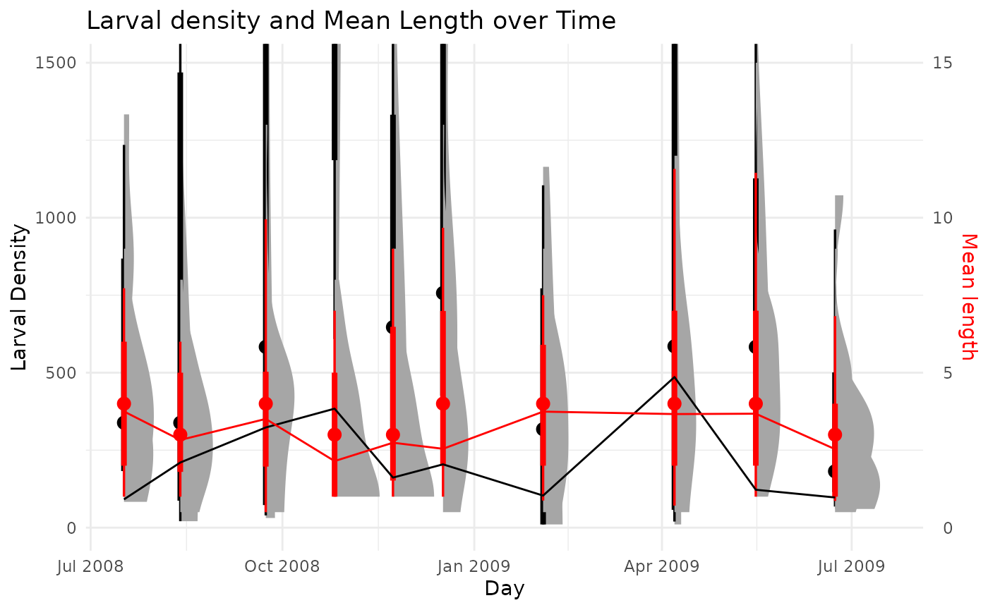
These figures can be helpful for identifying cohort structures and getting ballpark cohort production intervals (CPI) for species when estimating production using the size-frequency method. In this case, we see there is not much for distinguishable cohort structure, such as clear drops in density and concurrent increases in mass over time. Rather, there is a fairly consistent length structure and variable density over time.
We can also plot this taxa using mass as the size variable:
plot_cohorts(taxaSampleListMass = chiroMass,
             param = 'mass',
             massValue = 'mass',
             abunValue = 'n_m2')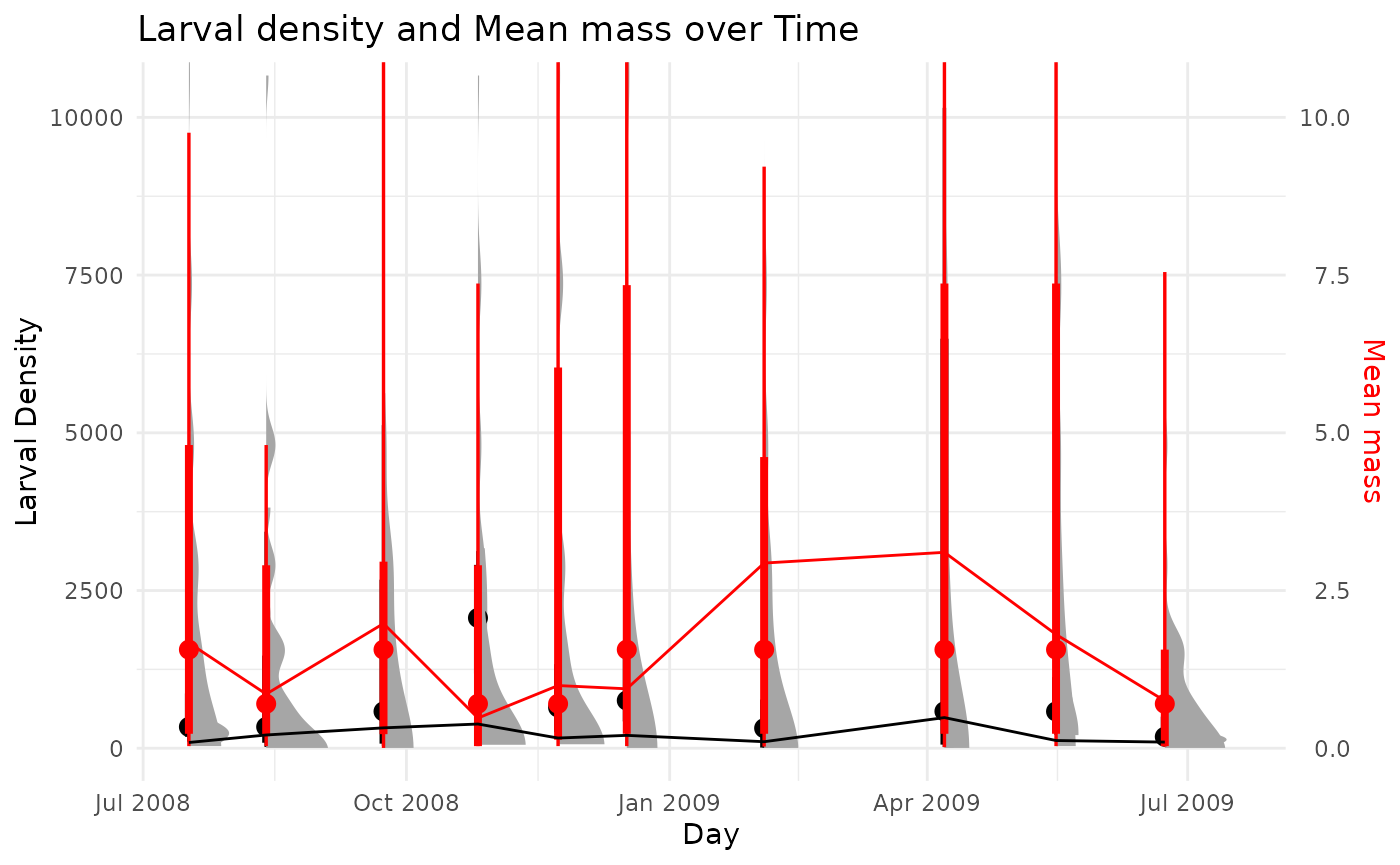
This shows a similar lack of structure. This is not surprising given the life history of this taxa. This suggest we should use a non-cohort method for estimating production in this case. Let’s use the instantaneous growth rate method, using the growth equation from Huryn (1990).
# setting the method to 'igr'

chiroInfo$method <- 'igr'
The function calc_production() is the workhorse function
that will estimate population or community production.
To apply it to our single species example, we input the sample
information and taxa information along with how many bootstraps we would
like. Further, because we are using the instantaneous growth method, we
also provide some environmental data to inform the growth rates, in this
case mean monthly temperature, tempC.
envData <- data.frame(
  dateID = as.Date(unique(unlist(chiroMass$dateID))),
  tempC = c(13.69,9.45,4.03,0.78,0.14,0.21,1.28,4,7.33,10.51)
  )

set.seed(1312)
calc_production(
  taxaSampleListMass = chiroMass,
  taxaInfo = chiroInfo,
  bootNum = 10,
  wrap = TRUE,
  taxaSummary = TRUE,
  lengthValue = 'lengthClass',
  massValue = 'mass',
  abunValue = 'n_m2',
  dateCol = 'dateID',
  repCol = 'repID',
  envData = envData
)
#> $P.boots
#>            [,1]     [,2]     [,3]     [,4]     [,5]     [,6]     [,7]
#> P.ann.samp 1977.99  2525.241 3105.415 2565.281 3130.709 2083.44  2514.561
#> B.ann.samp 828.494  1099.962 927.4515 955.3265 1147.914 775.4065 940.7444
#> N.ann.samp 918.7271 1208.345 1232.868 1146.944 1347.884 876.9376 1100.208
#>            [,8]     [,9]     [,10]
#> P.ann.samp 2491.577 3800.59  2293.374
#> B.ann.samp 862.0506 999.5042 744.874
#> N.ann.samp 1014.737 1193.647 1035.097
#>
#> $taxaSummary
#> $taxaSummary$taxonID
#> [1] "Chironomidae"
#>
#> $taxaSummary$method
#> [1] "igr"
#>
#> $taxaSummary$P.ann.samp
#> [1] 2464.977
#>
#> $taxaSummary$pb
#> [1] 2.844627
#>
#> $taxaSummary$meanN
#> [1] 1011.622
#>
#> $taxaSummary$meanB
#> [1] 866.5376
#>
#> $taxaSummary$meanIndMass
#> [1] 0.8565827
#>
#> $taxaSummary$datesInfo
#>        dateID  N n_m2_mean   n_m2_sd biomass_mean biomass_sd production
#> 1  2008-07-17 10  475.0000  408.6969     865.9706   912.5493  660.60224
#> 2  2008-08-13 10  861.6751 1212.5305     741.4426  1103.1644  595.43852
#> 3  2008-09-23 10 1357.5977 1837.5083     688.3785   552.1911  156.66332
#> 4  2008-10-26 10 1804.5430 1067.5783     962.2140   739.8756   87.41918
#> 5  2008-11-23 10  921.1053  869.1099     764.4288   563.0330   32.59893
#> 6  2008-12-17 10 1103.2950 1020.8328     939.2751  1340.2913   84.86127
#> 7  2009-02-03  8  401.1773  427.6119     308.7145   244.7629   52.93343
#> 8  2009-04-07 10 2818.0049 3896.7681    2167.6043  2701.3540  436.55304
#> 9  2009-05-16 10  709.5295  709.9744    1327.3375  1684.6170  211.71457
#> 10 2009-06-23 10  292.2737  320.8707     222.3751   238.1173  133.32871
#> 11 2009-07-16 NA  592.2648  819.2050    1096.6540  1915.9020   12.86336